现代计算机图形学入门

• 可选教材: Fundamentals of Computer Graphics(虎书 tiger book)
• 课程网址:GAMES101: 现代计算机图形学入门 (ucsb.edu)
• 计算机图形学与混合现实研讨会BBS:计算机图形学与混合现实在线平台 – GAMES: Graphics And Mixed Environment Symposium (games-cn.org)
• 闫令琪个人主页:Lingqi Yan: Research Homepage (ucsb.edu)

Course Topics

• Rasterization 光栅化

• Curves and Meshes 曲线和曲面

• Ray Tracing 光线追踪

• Animation / Simulation 动画与模拟

Review of Linear Algebra

• 判断内外可用叉乘

• 叉乘矩阵表示

  • $$
    \vec{a}\times\vec{b}=A^*b=
    \left(
    \begin{array}{c}
    0 & -z_a & y_a\
    z_a & 0 & -x_a\
    -y_a & x_a & 0
    \end{array}
    \right)
    \cdot
    \left(
    \begin{array}{c}
    x_b\
    y_b\
    z_b
    \end{array}
    \right)
    $$

引入Homogeneous Coordinates(齐次坐标)

• 目的是消除图像平移的特殊性，将所有变换转换成矩阵乘积形式

• 使用方法：加入第三个维度Add a third coordinite(w-coordinate)

  • 2D point = (x,y,1)^T (点)

  • 2D vector=(x,y,0)^T (向量)

  • 平移：

  • $$
    \left(
    \begin{array}{c}
    x’\
    y’\
    w’
    \end{array}
    \right)

    \left(
    \begin{array}{c}
    1 & 0 & t_x\
    0 & 1 & t_y\
    0 & 0 & 1
    \end{array}
    \right)
    \cdot
    \left(
    \begin{array}{c}
    x\
    y\
    1
    \end{array}
    \right)

    \left(
    \begin{array}{c}
    x+t_x\
    y+t_y\
    1
    \end{array}
    \right)
    $$

• Valid operation if w-coordinate of result is 1 or 0

  • vector + vector = vector
  • point - point = vector
  • point + vector = point
  • point + point = midpoint

• In homogeneous coordinates

  • $$
    \left(
    \begin{array}{c}
    x\
    y\
    w
    \end{array}
    \right)
    is ; the ; 2D ; point
    \left(
    \begin{array}{c}
    x/w\
    y/w\
    1
    \end{array}
    \right)
    , w \ne 0
    $$

• Affine map = linear map + translation

  • $$
    \left(
    \begin{array}{c}
    x’\
    y’
    \end{array}
    \right)

    \left(
    \begin{array}{c}
    a & b\
    c & d
    \end{array}
    \right)
    \cdot
    \left(
    \begin{array}{c}
    x\
    y
    \end{array}
    \right)
    +
    \left(
    \begin{array}{c}
    t_x\
    t_y
    \end{array}
    \right)
    $$

• Using homogenous coordinates

  • $$
    \left(
    \begin{array}{c}
    x’\
    y’\
    1
    \end{array}
    \right)

    \left(
    \begin{array}{c}
    a & b & t_x\
    c & d & t_y\
    0 & 0 & 1
    \end{array}
    \right)
    \cdot
    \left(
    \begin{array}{c}
    x\
    y\
    1
    \end{array}
    \right)
    $$

• 对于旋转来说

  • $$
    R_\theta =
    \left(
    \begin{array}{c}
    cos\theta & -sin\theta\
    sin\theta & cos\theta
    \end{array}
    \right)
    $$

  • $$
    R_{-\theta} =
    \left(
    \begin{array}{c}
    cos\theta & sin\theta\
    -sin\theta & cos\theta
    \end{array}
    \right) =
    R_\theta^T
    $$

  • $$
    R_{-\theta} = R_{\theta}^{-1} \quad(by;definition)
    $$

3D Transforms

• Use homogeneous coordinates again

  • 3D point = (x,y,z,1)^T
  • 3D vector = (x,y,z,0)^T

• In general, (x,y,z,w)(w!=0) is the 3D point (x/w,y/w,z/w)

• Use 4*4 matrices for affine transformations

• $$
  \left(
  \begin{array}{c}
  x’\
  y’\
  z\
  1
  \end{array}
  \right)

  \left(
  \begin{array}{c}
  a & b & c & t_x\
  d & e & f & t_y\
  g & h & i & t_z\
  0 & 0 & 0 & 1
  \end{array}
  \right)
  \cdot
  \left(
  \begin{array}{c}
  x\
  y\
  z\
  1
  \end{array}
  \right)
  $$

• Rotation around x-, y-, or z-axis

• $$
  R_x(\alpha)=
  \left(
  \begin{array}{c}
  1 & 0 & 0 & 0\
  0 & cos\alpha & -sin\alpha & 0\
  0 & sin\alpha & cos\alpha & 0\
  0 & 0 & 0 & 1
  \end{array}
  \right)
  $$

• tips: There is something strange about R_y

• $$
  R_y(\alpha)=
  \left(
  \begin{array}{c}
  cos\alpha & 0 & sin\alpha & 0\
  0 & 1 & 0 & 0\
  -sin\alpha & 0 & cos\alpha & 0\
  0 & 0 & 0 & 1
  \end{array}
  \right)
  $$

• $$
  R_z(\alpha)=
  \left(
  \begin{array}{c}
  cos\alpha & -sin\alpha & 0 & 0\
  sin\alpha & cos\alpha & 0 & 0\
  0 & 0 & 1 & 0\
  0 & 0 & 0 & 1
  \end{array}
  \right)
  $$

Rodrigues’ Rotation Formula罗德里格斯旋转公式

• Rotation by angle $\alpha$ around axis $\vec{n}$
  • $R(\vec{n},\alpha) = cos(\alpha)\vec{I} + (1-cos(\alpha))\vec{n}\vec{n^T} + sin(\alpha)\left(\begin{array}{c}0 & -n_z & n_y \ n_z & 0 & -n_x\-n_y & n_x & 0\end{array}\right)$ (右边这个矩阵刚好是叉乘矩阵)

四元数

Viewing(观测) transformation

• View(视图)/Camera transformation
• Projection(投影) transformation
  • Orthograpgic(正交) projection
  • Perspective(透视) projection

View/Camera Transformation

• How to take a photo

  • Find a good place and arrange people(model transformation)
  • Find a good “angle” to put the camera(view transformation)
  • Cheese!(projection transformation)

• Define the camera first

  • Position $\vec{e}$
  • Look-at / gaze direction $\hat{g}$
  • Up direction $\hat{t}$ (assuming perp. to look-at)

• Key observation

  • If the camera and all objects move together, the “photo” will be the same

• 

• 

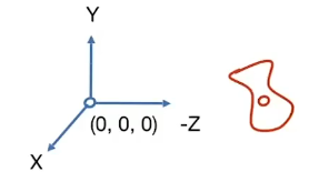
• How about that we always transform the camera to

  • The origin, up at Y, look at -Z
  • And transform the objects along with the camera

• Transform the camera by M_view

  • So it’s located at the origin, up at Y, look at -Z

• 

• M_view in math?

  • Translate e to origin
  • Rotates g to -Z
  • Rotates t to Y
  • Rotates (g x t) To X
  • Let’s write M_view=R_viewT_view 先平移再线性变换

  $$
  T_{view}=
  \left(
  \begin{array}{c}
  1 & 0 & 0 & -x_e\
  0 & 1 & 0 & -y_e\
  0 & 0 & 1 & -z_e\
  0 & 0 & 0 & 1
  \end{array}
  \right)
  $$

  • Translate e to origin

  • Rotate g to -Z, t to Y, (g $\times$ t) to X

  • Consider its inverse rotation: X to (g $\times$ t), Y to t, Z to -g

  • $R_{view}^{-1}$怎么得到的？

    • 举例：$X(1,0,0)^T\cdot R_{view}^{-1}=(\vec{g}\times\vec{t})$

  • $$
    R_{view}^{-1}=
    \left(
    \begin{array}{c}
    x_{\hat{g}\times\hat{t}} & x_t & x_{-g} & 0\
    y_{\hat{g}\times\hat{t}} & y_t & y_{-g} & 0\
    z_{\hat{g}\times\hat{t}} & z_t & z_{-g} & 0\
    0 & 0 & 0 & 1
    \end{array}
    \right)
    \rightarrow
    R_{view}=
    \left(
    \begin{array}{c}
    x_{\hat{g}\times\hat{t}} & y_{\hat{g}\times\hat{t}} & z_{\hat{g}\times\hat{t}} & 0\
    x_t & y_t & z_t & 0\
    x_{-g} & y_{-g} & z_{-g} & 0\
    0 & 0 & 0 & 1
    \end{array}
    \right)
    $$

  • 旋转矩阵是正交矩阵，所以他的逆就是他的转置。

• Summary

  • Transform objects together with the camera
  • Until camera’s at the origin, up at Y, look at -Z

• Also known as ModelView Transformation

Orthographic Projection

• A simple way of understanding

  • Camera located at origin,looking at -Z, up at Y
  • Drop Z coordinate
  • Translate and scale the resulting rectangle to [-1,1]²

• In general

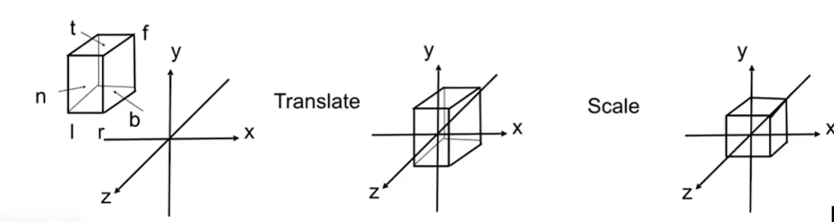
  • We want to map a cuboid [l,r]$\times$[b,t]$\times$[f,n] to the "canonical(正则、规范、标准)"cube [-1,1]³

  • 

  • Slightly different orders (to the “simple way”)

    • Center cuboid by translation
    • Scale into “canonical” cube

  • Translate (center to origin) first, then scale (length/width/height to 2)

  • $$
    M_{ortho}=
    \left(
    \begin{array}{c}
    \frac{2}{r-l} & 0 & 0 & 0\
    0 & \frac{2}{t-b} & 0 & 0\
    0 & 0 & \frac{2}{n-f} & 0\
    0 & 0 & 0 & 1
    \end{array}
    \right)
    \cdot
    \left(
    \begin{array}{c}
    1 & 0 & 0 & -\frac{r+l}{2}\
    0 & 1 & 0 & -\frac{t+b}{2}\
    0 & 0 & 1 & -\frac{n+f}{2}\
    0 & 0 & 0 & 1
    \end{array}
    \right)
    $$

Perspective Projection

• Most common in Computer Graphics, art, visual system

• Further objects are smaller

• Parallel lines not parallel; converge to single point

• How to perspective projection

  • First “squish” the frustum into a cuboid(n->n,f->f)($M_{persp->ortho}$)
  • Do orthograpgics projection($M_{ortho}$ ,already know!)

• In order to find a transform

  • Recall the key idea: Find the relationship between transformed points(x’,y’,z’) and the original points(x,y,z)
  • 
  • $x’ = \frac{n}{z}x$ {similar to y’}

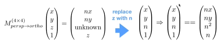
• In homogeneous coordinates

  • 

• So the “squish” (persp to ortho) projection does this

  • $$
    M_{persp\rightarrow ortho}
    \left(
    \begin{array}{c}
    x\
    y\
    z\
    1
    \end{array}
    \right)=
    \left(
    \begin{array}{c}
    nx\
    ny\
    unknown\
    z
    \end{array}
    \right)
    $$

• Already good enough to figure out part of $M_{persp\rightarrow ortho}$

  • $$
    M_{persp\rightarrow ortho}=
    \left(
    \begin{array}{c}
    n & 0 & 0 & 0\
    0 & n & 0 & 0\
    ? & ? & ? & ?\
    0 & 0 & 1 & 0
    \end{array}
    \right)
    $$

  • Any information that we can user?

• Observation: the third row is responsible for z’

  • Any point on the near plane will not change
  • Any point’s z on the far plane will not change
  • 

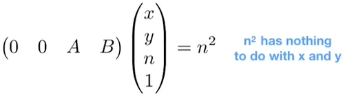
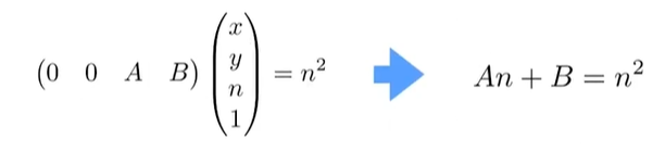
• So the third row must be of the form(0 0 A B)

  • 

• What do we know now?

  • 

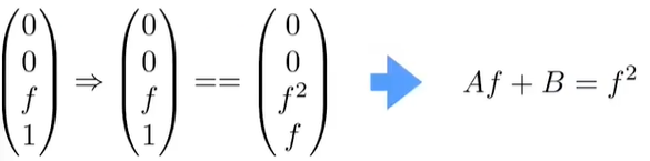
• Any point’s z on the far plane will not change

  • 

• Solve for A and B

  • 

• Finally, every thing in $M_{persp\rightarrow ortho}$ is known!

• What’s next?

  • Do orthographic projection(M_ortho) to finish
  • $M_{persp}=M_{ortho}M_{persp\rightarrow ortho}$

一、Rasterization 光栅化

• 光栅化：
  • 把三维空间的几何实体显示在屏幕上

Canonical Cube to Screen

• Irrelevant to z

• Transform in xy plane: [-1,1]² to [0,width]$\times$[0,height]

• Viewport transform matrix

  • $$
    M_{persp\rightarrow ortho}=
    \left(
    \begin{array}{c}
    \frac{width}{2} & 0 & 0 & \frac{width}{2}\
    0 & \frac{height}{2} & 0 & \frac{height}{2}\
    0 & 0 & 1 & 0\
    0 & 0 & 0 & 1
    \end{array}
    \right)
    $$

Sampling Artifacts in Computer Graphics

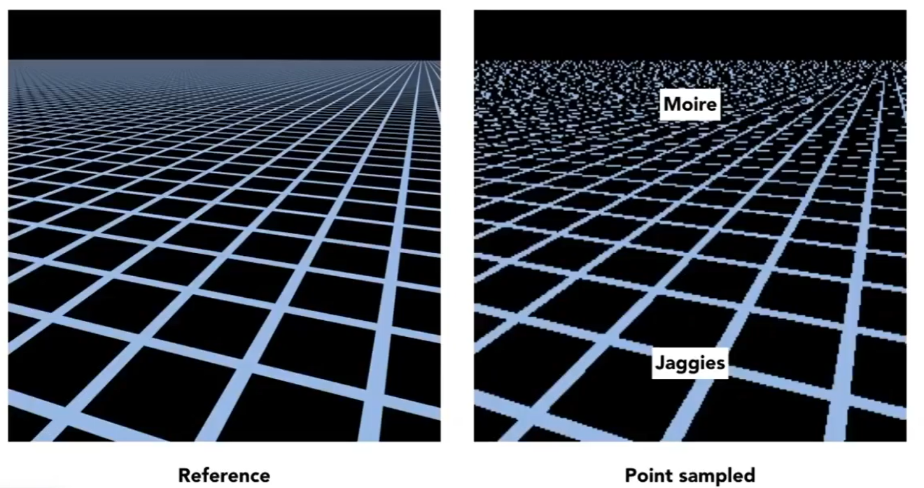
• Artifacts due to sampling - “Aliasing”

  • Jaggies - samping in space

  • Moire - undersampling images

  • Wagon wheel effect - sampling in time

  • [Many more]…

• Behind the Aliasing Artifacts

  • Signals are changing too fast(high frequency) but sampled too slowly

Antialiasing

Antialiasing Idea: Blurring(Pre-Filtering) Before Sampling

Sampling theory

Antialiasing in practice

• MSAA(By Supersampling)

• FXAA(Fast Approximate AA)

• TAA(Temporal AA)

• Super resolution / super sampling

  • From low resolution to high resolution
  • Essentially still “not enough samples” problems
  • DLSS(Deep Learning Super Sampling)

Visibility/occlusion

Z-buffering

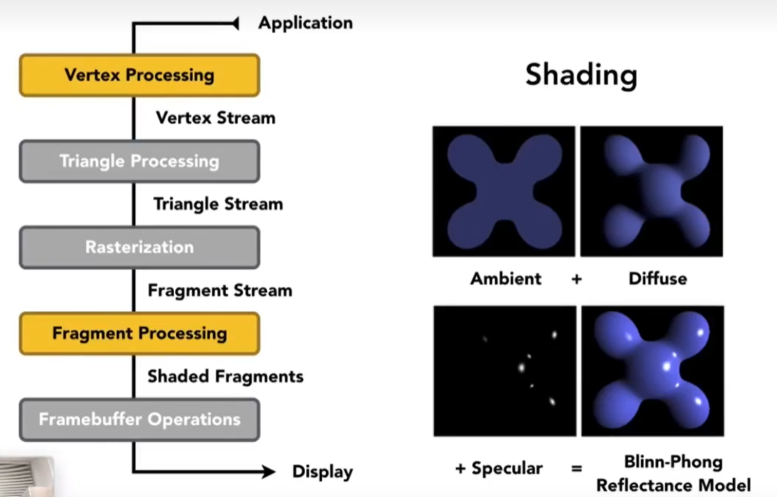
二、Shading

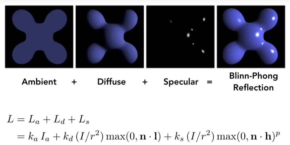
A Simple Shading Model(Blinn-Phong Reflectance Model)

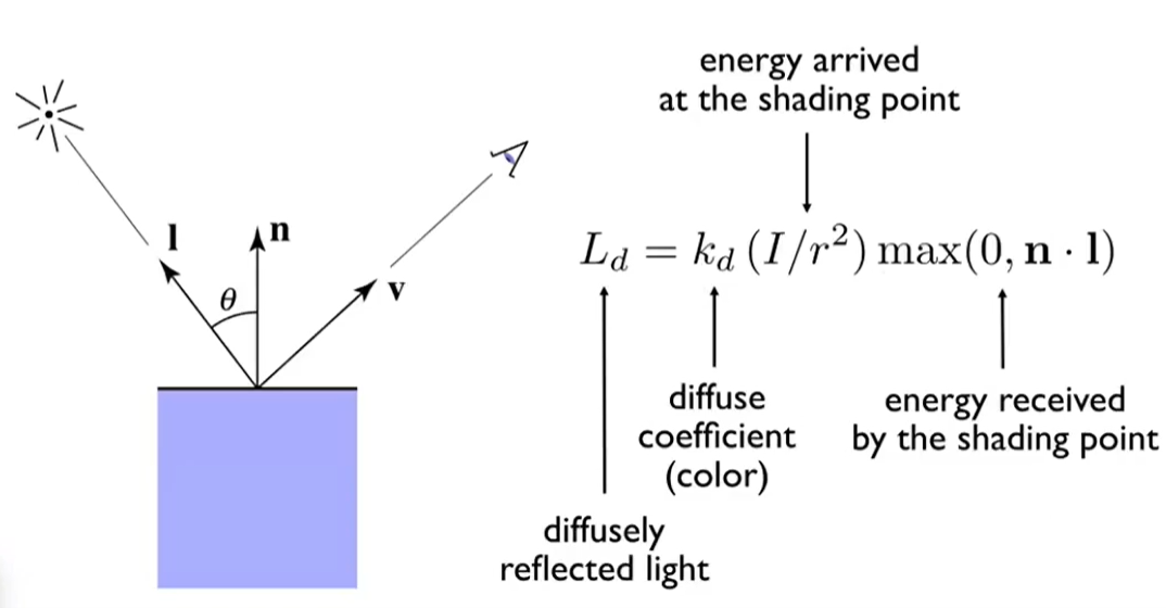
Diffuse Reflection

• Lambert’s cosine law

• Shading independent of view directing 漫反射出去的光朝四面八方都一样，与v无关

Specular reflection

• Intensity depends on view direction

  • Bright near mirror reflection direction镜面反射方向最亮

• V close to mirror direction 相似 half vector near normal

  • Measure “near” by dot product of unit vectors

  

  • 上面的指数p 是根据角度与余弦值关系加上的，减小容忍度。Incresing p narrows the reflection lobe. P越大，高光范围越小

Ambient Reflection

• Shading that does not depend on anything

  • Add constant color to account for disregarded illumination and fill in black shadows
  • This is approximate / fake!

  

• 所有项加起来

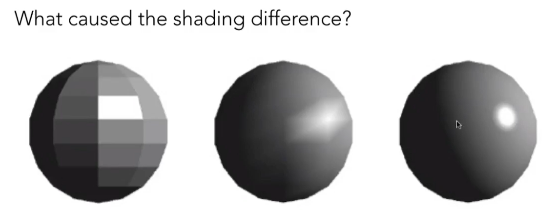
Shading Frequencies

• 从左到右

  • Flat Shading每个平面计算一个法线

    • Triangle face is flat - one normal vector
    • Not good for smooth surfaces

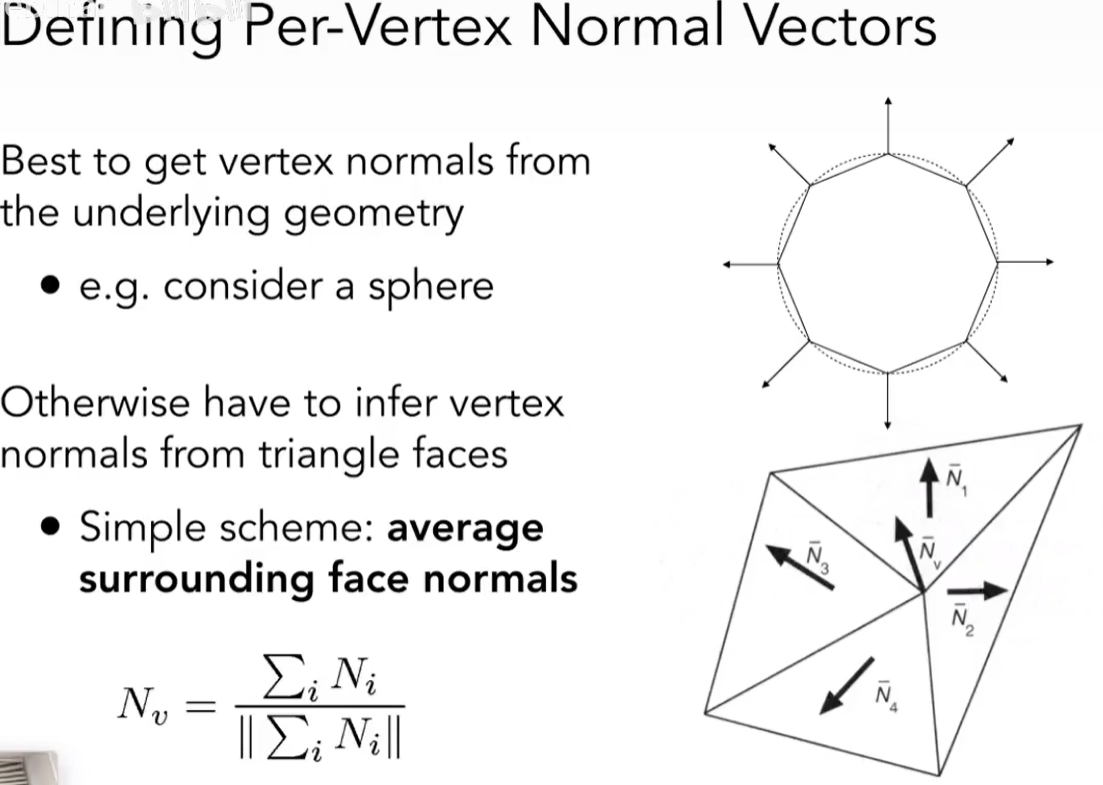
  • Gouraud shading每个顶点计算一个法线然后做插值

    • Interpolate colors from vertices across triangle
    • Each vertex has a normal vector(how?)

    

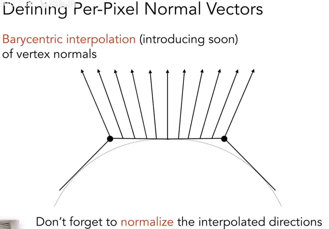
  • Phong shading每个像素计算一个法线

    • Interpolate normal vectors across each triangle
    • Compute full shading model at each pixel
    • Not the Blinn-Phong Reflectance Model

    

Graphics(Real-time Rendering) Pipeline

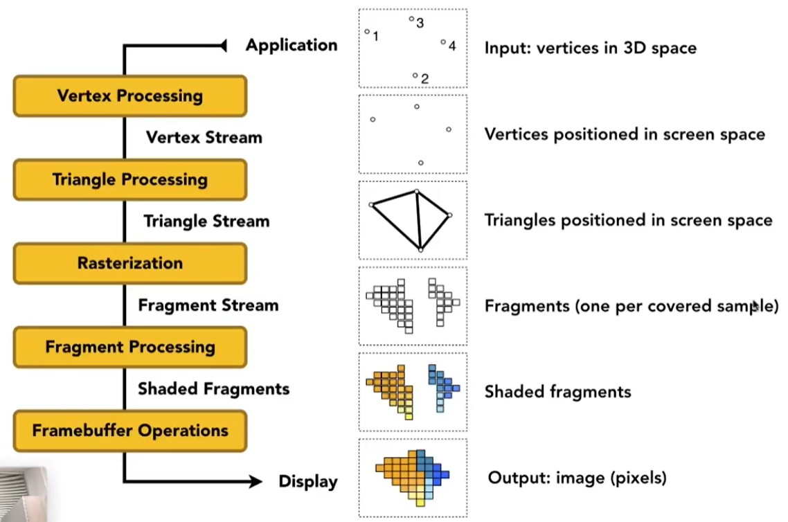
注意:shading的地方:

• 如果是顶点着色，就可以发生在Vertex Processing
• 如果是Phong着色，就会发生在Fragment Processing

Shader Programs

• Program vertex and fragment processing stages
• Describe operation on a single vertex(or fragment)
• Example GLSL fragment shader program
• 
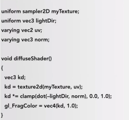
  • Shader function executes once per fragment.
  • Outputs color of surface at the current fragment’s screen sample position.
  • This shader performs a texture lookup to obtain the surface’s material color at this point, then performs a diffuse lighting calculation.

Texture Mapping

Interpolation Across Triangles Barycentric Coordinates(中心坐标)

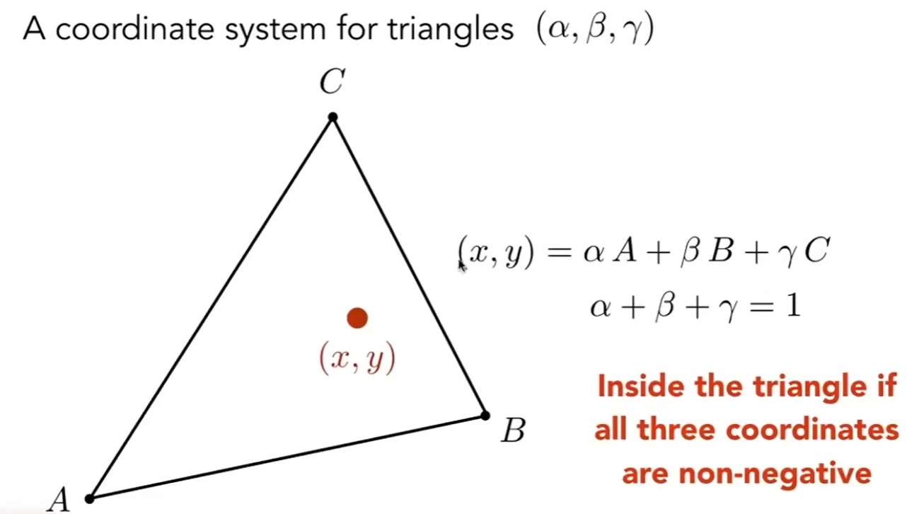
• 三个系数如果都是非负的，则中心坐标一定在三角形内。

• 重心坐标三个系数都是三分之一

• 投影前计算出来的中心坐标无法投影到投影后计算出的中心坐标(要在投影之前计算出来重心)

Applying Texture

Texture Magnification(What if the texture is too small?) - Easy Case(纹理比图像分辨率小的问题)

Generally don’t want this - insufficient texture resolution

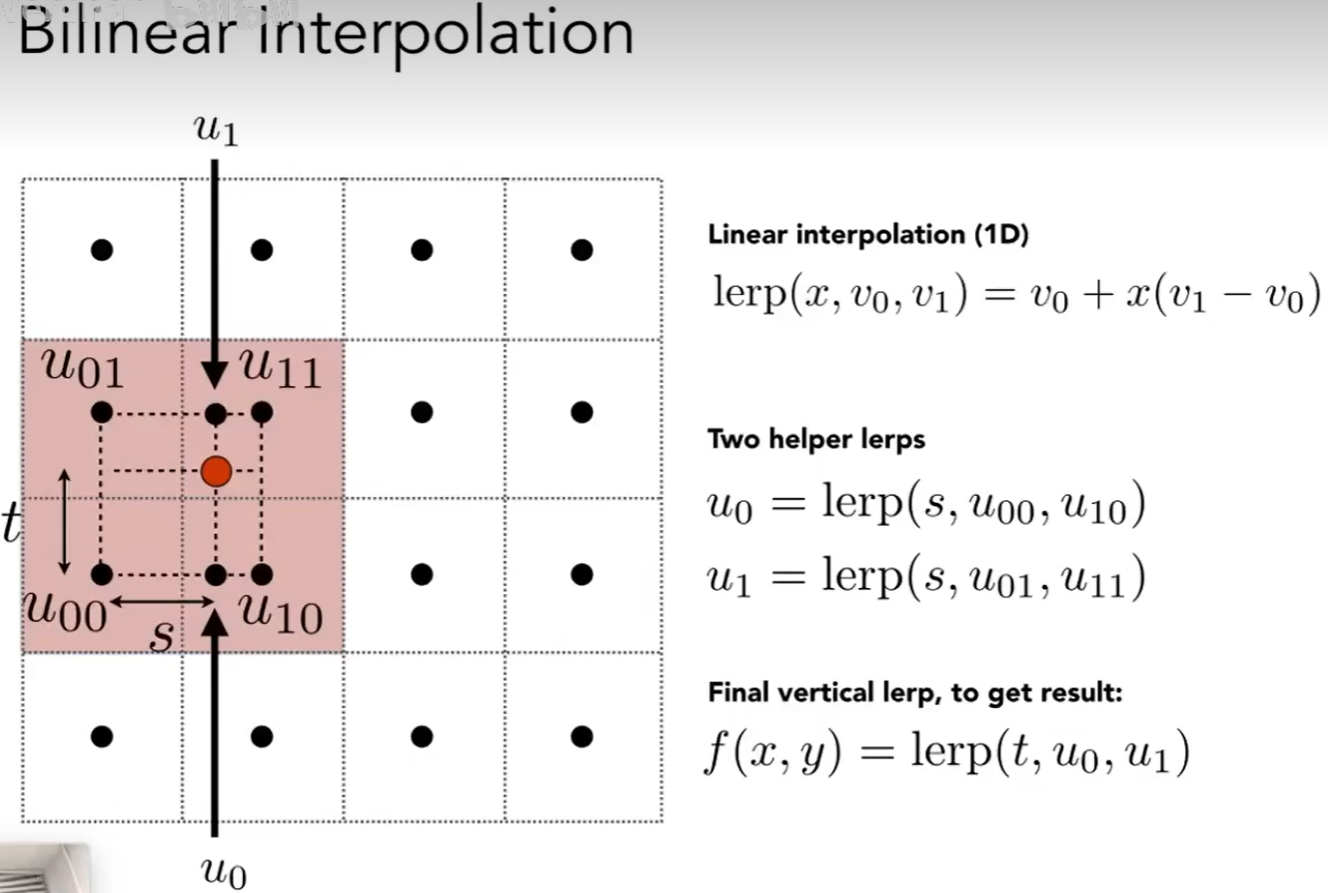
A pixel on a texture - a texel(纹理元素、纹素)

• 双线性插值
  • Bilnear interpolation usually gives pretty good results at reasonable costs

Texture Magnification(What if the texture is too large) - hard case(纹理比图像分辨率大的问题)

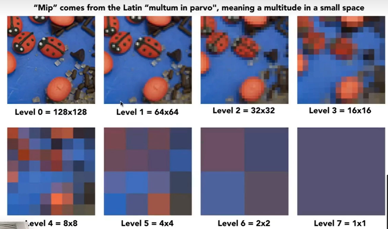
Mipmap Allowing(fast,approx.,square) range queries

• 额外的三分之一存储

Computing Mipmap Level D

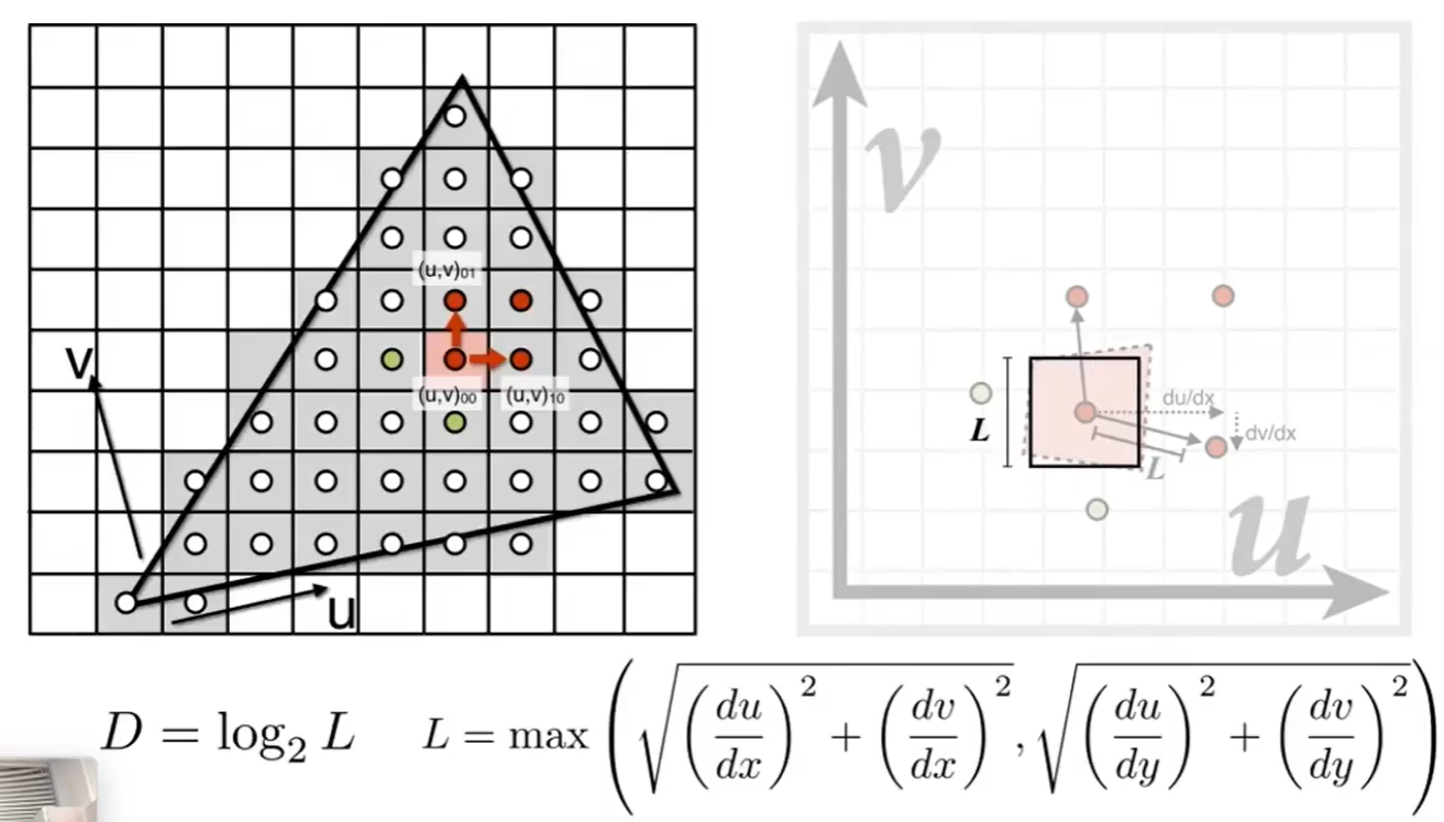
• 对映射过去的正方形做近似，应用Mipmap Allowing将矩形变成第D层的1$\times$1矩形，映射到一个像素中

Visualization of Mipmap Level

• 单纯的映射效果不好，因为mipmap取层数是离散的，会出现间断的线

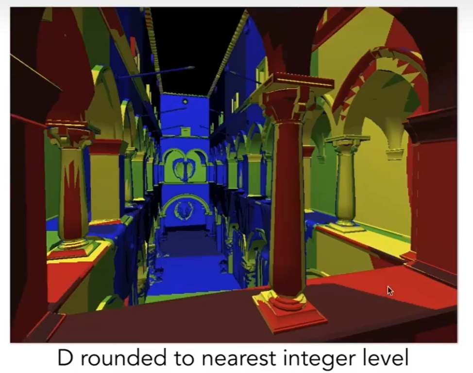
因此可做一次三线性插值，取连续插值层texel(纹理元素，纹素)

Trilinear Interpolation

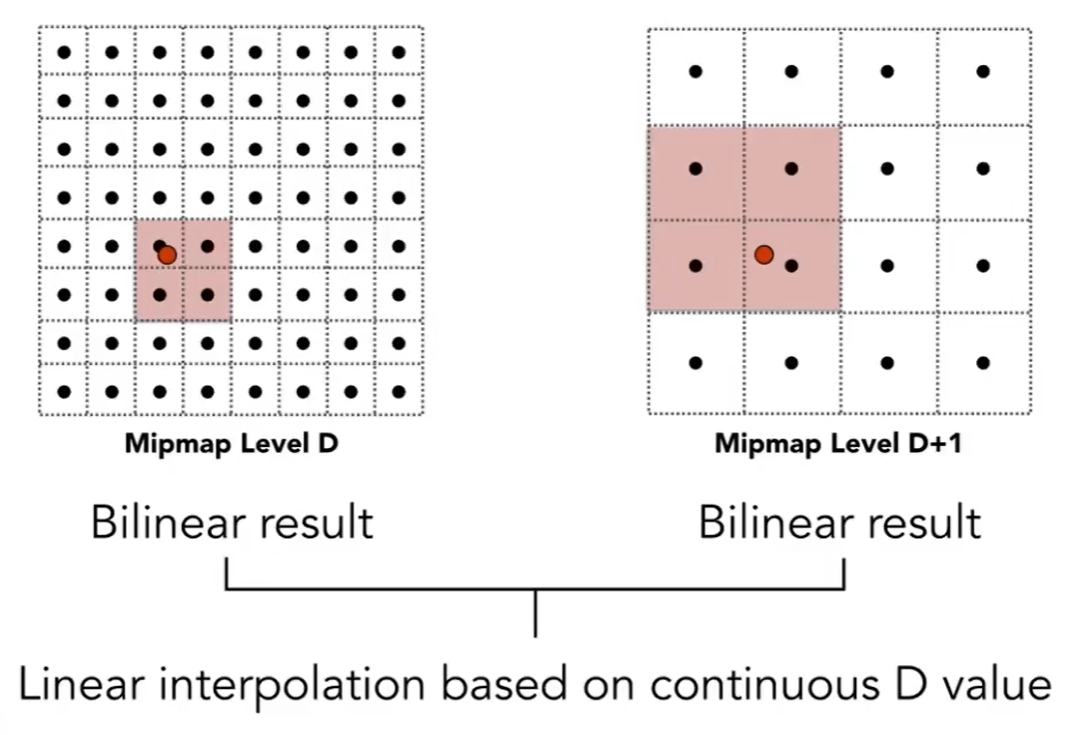
• 在相邻两层中各做双线性插值，然后将结果再做一次线性插值。

• 但这样做效果并不好，远处的细节都会模糊(Overblur)，使用下面来改善

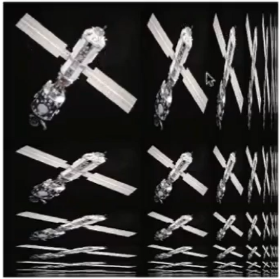
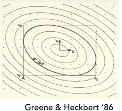
Anisotropic Filtering(各向异性过滤)

Ripmaps and summed area tables

• Can look up axis-aligned rectangular zones
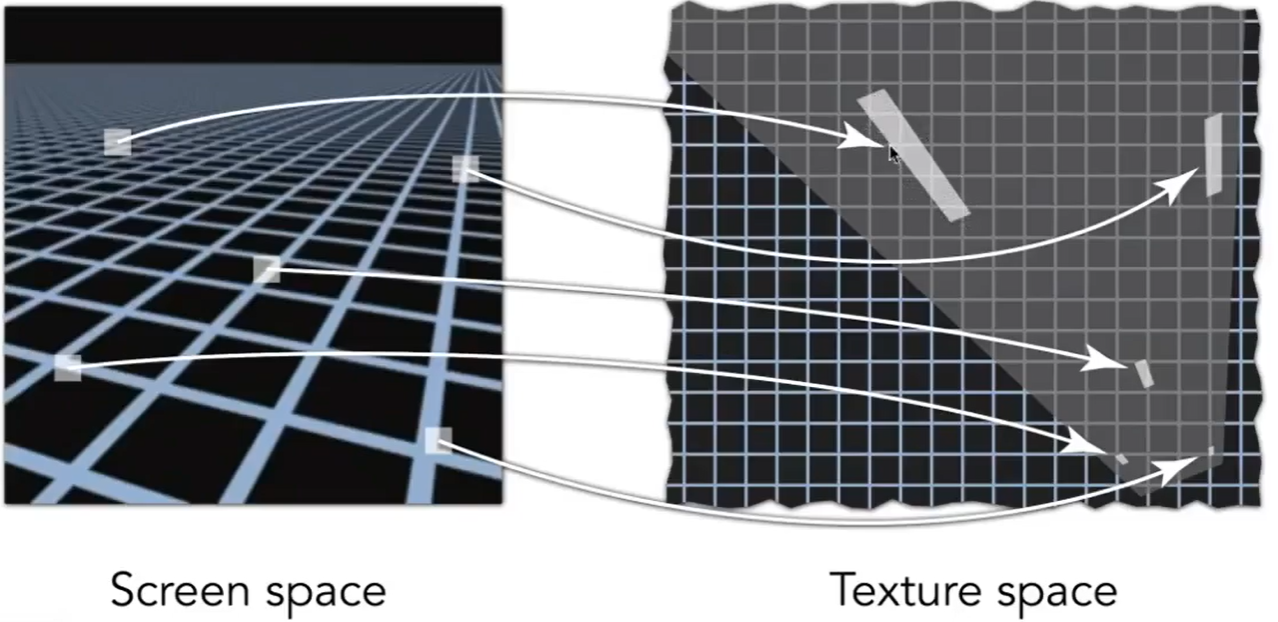
• Diagonal footprints still a problem

Irregular Pixel Footprint in Texture(不用水平竖直都压缩，可以只压缩一个方向),但是还有一些情况没能解决，比如映射过去覆盖的是一种斜着的长条

EWA filtering

• Use multiple lookups
• Weighted average
• Mipmap hierarchy still helps
• Can handle irredular footprints

Many, Many Uses for Texturing

In modern GPUs, texture = memory + range query(filtering)

• General method to bring data to fragment calculations

Textures can affect shading!

• Texture doesn’t have to only represent colors
  • What if it stores the height/normal?
  • Bump / normal mapping
  • Fake the detailed geometry

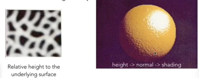
Bump Mapping

Adding surface detail without adding more triangles

• Perturb surface normal per pixel(for shading computations only)

• “Height shift” per texel defined by a texture

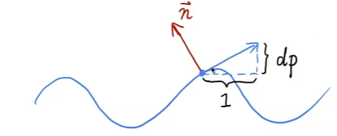
• How to modify normal vector?

How to perturb the normal(in flatland)

• Original surface normal n§ = (0,1)
• Derivative at p is dp = c * [h(p+1) - h§]
• Perturbed normal is then n§ = (-dp,1).normalized()

How to perturb the normal (in 3D)

• Original surface normal n§ = (0,0,1)
• Derivatives at p are
  • dp/dv = c1* [h(u+1) - h(u)]
  • dp/dv = c2 * [h(v+1) - h(v)]
• Perturbed normal is n = (-dp/du, -dp/dv,1).normalized()
• Note that this is in local coordinate!

Displacement mapping

a more advanced approach

• Uses the same texture as in bumping mapping
• Actually moves the vertices

三、Geometry

Many Ways to Represent Geometry

• Implicit
  • algebraic surface
  • level sets
  • distance functions
• Explicit
  • point cloud
  • polugon mesh
  • subdivision,NURBS

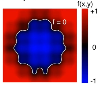
“Implicit” Representations of Geometry

Based on classifying points

• Points satisfy some specified relationship

E.g. sphere: all points in 3D,where x²+y²+z²=1

More generally,f(x,y,z) = 0

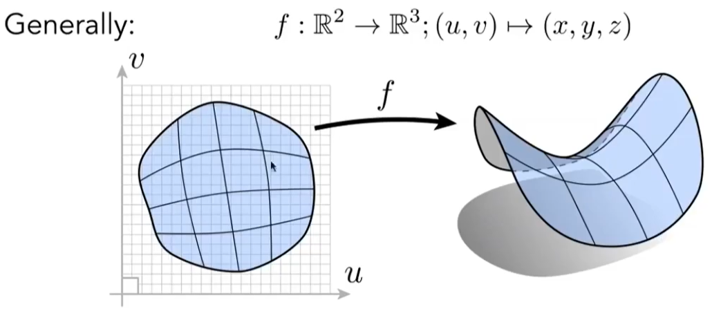
“Explicit” Representations of Geometry

All points are given directly or via parameter mapping

Implicit

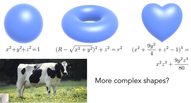
Algebraic Surfaces(Implicit)

Surface is zero set of a polynomial in x,y,z

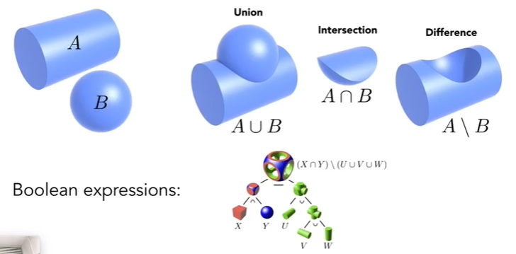
Constructive Solid Geometry(Implicit)

Combine implicit geometry via Boolean operations

Distance Fuctions(Implicit)

Instead of Booleans, gradually blend surfaces together using

• Distance fuctions:

  giving minimum distance(could be signed distance) from anywhere to object

Level Set Methods

Closed-form equations are hard to describe complex shapes

Alternative: store a grid of values approximating function

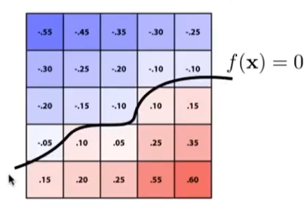
Surface is found where interpolated values equal zero

Provides much more explicit control over shape(like a texture)

Fractals(Implicit)(分形)

Exhibit selt-similarity, detail at all scales

“Language” for describing natural phenomena

Hard to control shape!

Implicit Representations - Pros & Cons

• Pros:
  • compact description(e.g., a fuction)
  • certain queries easy(inside object, distance to surface)
  • good for ray-to-surface intersection(more later)
  • for simple shapes, exact description / no sampling error
  • easy to handle changes in topology(e.g., fluid)
• Cons:
  • difficult to model complex shapes

Explicit

Point Cloud

Easiest representation: list of points(x,y,z)

Polygon Mesh

Store vertices & polygons(often triangles or quads)

Easier to do processing/simulation,adaptive sampling

More complicated data structures

Perhaps most common representation in graphics

Curves

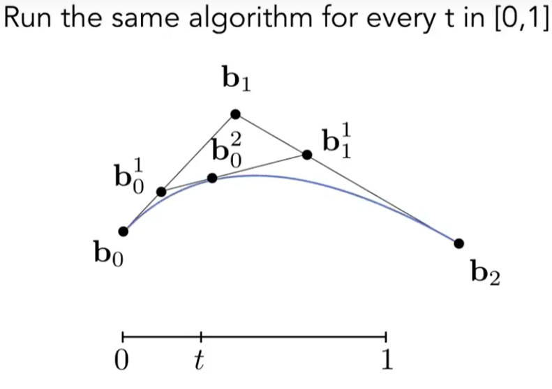
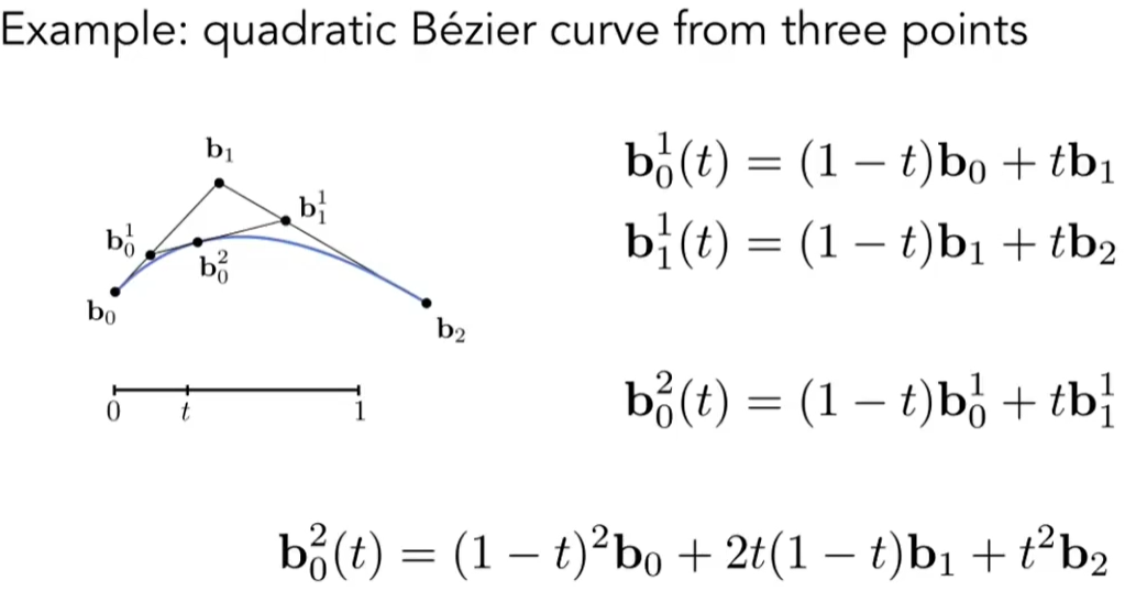
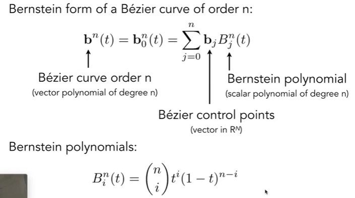
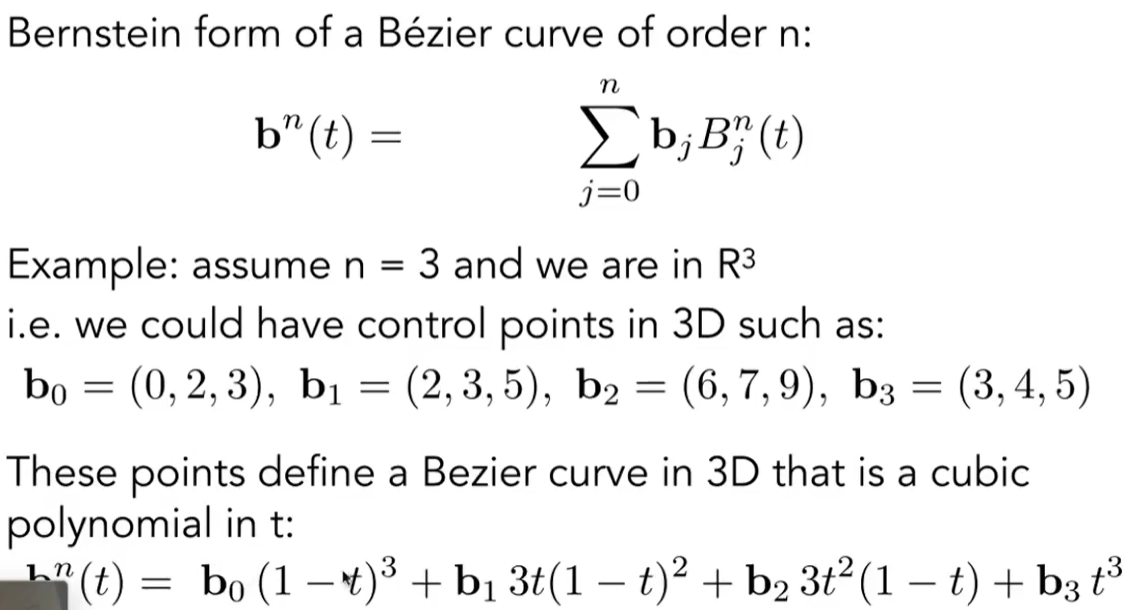
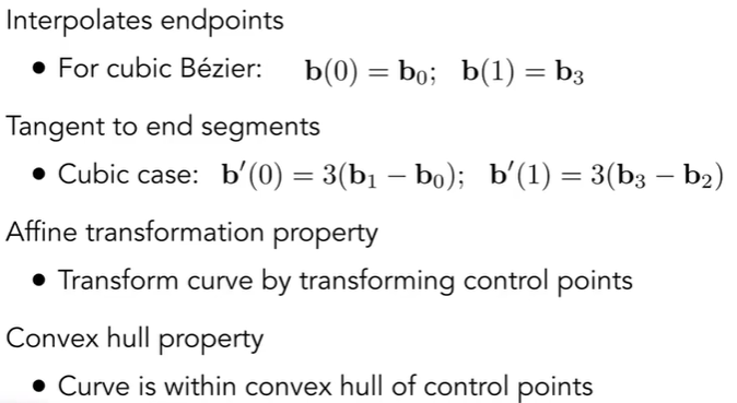
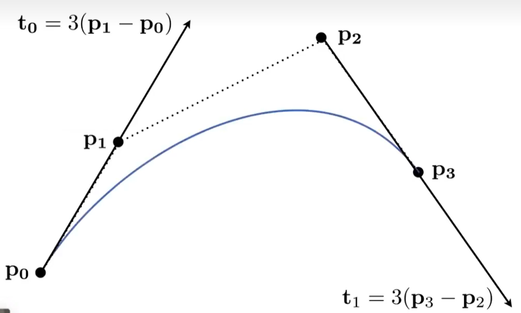
Bezier Curves(贝塞尔曲线)

• Defining Cubic Bezier Curve With Tangents

曲线要经过起止点

• de Casteljau Algorithm